|
Kerasはニューラルネットワークの学習を容易にすために開発されたライブラリです。2015年に開発が開始されたKerasはTheanoをベースとして構築され、広く利用されているPythonで書かれたライブラリになっている。現在、Theano、Tensorflow及びCNTKなどをバックエンドとして利用できます。Kerasの標準インストールで、デフォルトでは、Tensorflowがバックエンドになっています。ディープラーニング用のライブラリであるKerasから、バックエンドとしてTensorFlow及びTheanoを用いたディープラーニングの実際の課題に挑戦します。
KerasはPythonで書かれていますので、Pythonの基礎的な知識を持っている人を想定します。なお、anaconda等でPythonのモジュール一式がインストールされていることも前提とします。deep-learningの理論的な説明は、例えば、3層パーセプトロン(MLP)や畳み込みニューラルネットワーク(CNN)の説明は、Deep Learningと人工知能のページにありますので、併せて読むと理解が深まると思います。
Kerasを活用するための日本語版ドキュメントはこのサイトにあります。このKeras.ioのドキュメントには、活用できるexamplesが多数掲載されています。
Keras (κέρας) はギリシア語で角を意味します.古代ギリシア文学およびラテン文学における文学上の想像がこの名前の由来です。Kerasは当初プロジェクトONEIROS (Open-ended Neuro-Electronic Intelligent Robot Operating System) の研究の一環として開発されました。
Kerasと類似の機能を持つライブラリにChainerがあります。しかし、ChainerはインストールするPCのOSとしてUbuntuが推奨されています。Mac OSで動作することは確認していますが、公式ホームページでは正常に作動することを保証していません。このページではMac OS(Mojave)をベースに説明しているので、Chainerを用いたCNNの実装手続きについては説明しません。OSとしてUbuntu16.04を用いたPCでも、このページで説明される手続きで、正常に動作することも確認しています。このページで必要なすべてのソースコードは私のGitHub Repositoryにありますので、ダウンロードして利用してください。
なお、2019年4月2日時点では、使用されているソフトウエアの環境は以下の通りにアップグレードされています。
numpyのバージョン:1.16.1
scipyのバージョン:1.1.0
matplotlibのバージョン:2.2.2
PIL(Pillow)のバージョン:5.1.0
kerasのバージョン:2.2.4
tensorflowのバージョン:1.13.1
です。
動作確認はTensorflow 1.13やKeras 2.24のバージョンで行っています。しかし、KerasやTensorflowのバージョンアップなどが行われた環境ではエラーなどが出て正常に作動しない可能性もありますので、ご注意ください。
なお、Tensorflow 2.0では、KerasがTensorFlowに統合され、tensorflow.contribモジュールが廃止されました。この結果、このページで取り上げたKerasのコードはTensorflow 1.xバージョンでは正常に作動しますが、Tensorflow 2.0では多くのプログラムは作動しません。Tensorflow 2.0を用いた機械学習ライブラリの実装については、TensorFlow 2.0 を用いた機械学習のページに解説が掲載されています。
Last updated: 2019.11.15
Tensorflow と Keras のインストール |
Anaconda3がインストールされていることを前提にします。Mac OS Mojave以下に対応するパッケージはこのanaconda3になります。また、anaconda3以下にインストールされているPythonモジュールへのパスが設定されているとします。anaconda3がインストールされるときには、このパスの設定は自動的に済んでいるはずです。以下のようなコマンドを入力してインストールします。kerasをインストールする前に必ず、バックエンドのtensorflowをインストールします。
$ conda install tensorflow==1.13この入力で、TensorFlowのパッケージは ~/anaconda3/lib/python3.6/site-packages/tensorflow/にインストールされます。このインストール方法 (Installing with native pip) でダメなときは、
sudo pip3 install --upgrade https://storage.googleapis.com/tensorflow/mac/cpu/tensorflow-1.10.1-py3-none-any.whlと入力してください。anaconda3ディレクトリの中にPython関連の必要な全てのパッケージが収容されます。
$ conda create -n tensorflow pip python=3.6
 (targetDirectory)$ source activate tensorflow
 (targetDirectory)$ pip install --ignore-installed --upgrade https://storage.googleapis.com/tensorflow/mac/cpu/tensorflow-1.8.0-py3-none-any.whl
(targetDirectory)はanaconda3以下のtensorflowがインストールされるディレクトリのことです。このケースでは、tensorflowを利用するときは必ず、$ source activate tensorflow を入力し、終了時には$ deactivate と入力して、homeディレクトリに戻しておく必要があります。詳しくは、公式サイトを参照してください。
$ python3
>>> import tensorflow as tf
>>> hello = tf.constant('Hello, TensorFlow!')
>>> sess = tf.Session()
>>> print(sess.run(hello))
$ pip uninstall tensorflow
$ pip install tensorflow==1.5
のようにバージョンを1.5にします。
$ conda install keras
Using TensorFlow backend.
scikit-learnのバージョンは0.19.1です
numpyのバージョンは1.14.3です
scipyのバージョンは0.19.1です
matplotlibのバージョンは2.1.0です
PIL(Pillow)のバージョンは4.2.1です
kerasのバージョンは2.1.5です
theanoのバージョンは1.0.1です
tensorflowのバージョンは1.8.0です
MacBook-Air:keras koichi$ ls
__init__.py
__pycache__
activations.py
applications
backend
callbacks.py
constraints.py
datasets
engine
initializers.py
layers
legacy
losses.py
metrics.py
models.py
objectives.py
optimizers.py
preprocessing
regularizers.py
utils
wrappers
Kerasの中心的なデータ構造はmodelで,レイヤーを構成する方法です。 主なモデルはSequentialモデルで,各レイヤーを線形に積み上げていくネットワークモデルです。更に複雑なアーキテクチャの場合は,Keras functional APIを使用する必要があります。このAPIを活用すると、任意の複雑なネットワーク・グラフが構築可能になります。
$ conda install h5pyさらに、構成したモデルを可視化して、そのグラフを描画するためには、graphvizとpydotを利用する必要があります。それらのパッケージは
$ conda install graphviz
$ conda install pydot
と入力してインストールします。これらのパッケージをインストールするに際して、コマンドにcondaを用いて、pip を使用しないのは、anaconda3ディレクトリの中にこれらのパッケージを失敗せずにインストールするためです。pipコマンドを用いても、使用するpcの環境設定に依存して、anaconda3ディレクトリ内にインストールされることはあります。
Sequentialモデルを用いた画像識別の例 |
Sequential モデルを用いた最も単純な例は以下のように書けます。
from keras.models import Sequential
from keras.layers import Dense

model = Sequential()
model.add(Dense(units=64, activation='relu', input_dim=100))
model.add(Dense(units=10, activation='softmax'))

model.compile(loss='categorical_crossentropy',
              optimizer='sgd',
              metrics=['accuracy'])

# visualize the network
from keras.utils import plot_model
plot_model(model, to_file='model.png')

# x_train and y_train are Numpy arrays --just like in the Scikit-Learn API.
model.fit(x_train, y_train, epochs=5, batch_size=32)
model = Sequential()で、Sequentialモデルを用いた具体的なモデル名をmodelとします。.add()メソッドで簡単にネットワークのレイヤーを積み重ねて、モデルを構築します。Dense(units=64, activation='relu', input_dim=100)は、第1の層が64個のニューロンが隣接する層と全結合されたレイヤで、活性化関数がRelu関数、入力データの配列次数が100であることを意味します。Dense(units=10, activation='softmax')は、追加される第2層が10個のニューロンからなる全結合層で、活性化関数がsoftmax関数であることを示します。from keras.utils import plot_model plot_model(model, to_file='model.png')をmodel.compile()の後において、実行してください。'model.png'という画像ファイルがcurrent directoryに生成されます。また,pydot.Graphオブジェクトを直接操作して可視化もできます. Jupyter Notebook内で
from IPython.display import SVG
from keras.utils.vis_utils import model_to_dot

SVG(model_to_dot(model).create(prog='dot', format='svg'))
というプログラムを実行します。
Functional APIモデルを用いた画像識別の例 |
functional APIを使ったシンプルな例を見てきましょう。
Sequentialモデルと異なる最初の一つは、layerを定義する前に、inputs=Input(...)と入力シェイプを指定する必要があります。レイヤーのインスタンス(ここでは、x=Dense(..))は関数(Denseなど)で呼び出し可能で,戻り値としてテンソルを返します。Modelでinputsとoutputsを定義することで、各レイヤーが接続されて、入力と出力のテンソルが接続されます。定義したモデルはSequentialと同様に、呼び出して利用可能です。以下のコードを見てください。MNISTデータをSequentialモデルで分類したものと類似のプログラムになります。ただし、3層パーセプトロンとなっています。
from keras.layers import Input, Dense
from keras.models import Model

# This returns a tensor
inputs = Input(shape=(784,))

# a layer instance is callable on a tensor, and returns a tensor
x = Dense(64, activation='relu')(inputs)
x = Dense(64, activation='relu')(x)
predictions = Dense(10, activation='softmax')(x)

# This creates a model that includes
# the Input layer and three Dense layers
model = Model(inputs=inputs, outputs=predictions)
model.compile(optimizer='rmsprop',
              loss='categorical_crossentropy',
              metrics=['accuracy'])
model.fit(data, labels)  # starts training
x = Input(shape=(784,))
# This works, and returns the 10-way softmax we defined above.
y = model(x)
とします。詳しい説明は、公式サイトKeras.ioを参照ください。
簡単なSequentialモデルを用いた手書き数字の識別 |
それでは、実際にモデルを実装してみましょう。ディープラーニングでテストデータとして頻繁に登場するMNISTを使用します。MNISTデータは、アメリカ国立標準技術研究所(NIST)が用意した手書き数字の画像データベースで、機械学習の分野で画像認識の入門用サンプルとして利用されている。MNISTデータを読み込むために、以下のコードを作成ましょう。Jupyter Notebookを起動して、「+」をクリックして、そこに以下のコードをコピペしてください。以下で使用するコードの多くは、github Keras-teamから引用したものを部分的に修正したものです。
from __future__ import print_function
import keras
from keras.datasets import mnist
import matplotlib.pyplot as plt
# Kerasのmnist関数でデータの読み込み。
# 訓練データ(x_train, y_train)とテストデータ(x_test, y_test)に分割
(x_train, y_train), (x_test, y_test) = mnist.load_data()
# MNISTデータの表示
fig = plt.figure(figsize=(9, 9))
fig.subplots_adjust(left=0, right=1, bottom=0, top=0.5, hspace=0.05, wspace=0.05)
for i in range(81):
ax = fig.add_subplot(9, 9, i + 1, xticks=[], yticks=[])
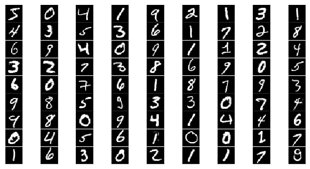
ax.imshow(x_train[i].reshape((28, 28)), cmap='gray')
このセルを実行すると、手書き数字のサンプルが表示されます。データは教師ラベル付けされた10種類の手書き数字の白黒画像(画素数は28x28 pixels=784)です。訓練データが60000枚、テストデータが10000枚となっている。(y_train,y_test)が教師ラベル(正解)です。
num_classes = 10
x_train = x_train.reshape(60000, 784)
x_test = x_test.reshape(10000, 784)
x_train = x_train.astype('float32')
x_test = x_test.astype('float32')
x_train /= 255
x_test /= 255

y_train = y_train.astype('int32')
y_test = y_test.astype('int32')
y_train = keras.utils.np_utils.to_categorical(y_train, num_classes)
y_test =  keras.utils.np_utils.to_categorical(y_test, num_classes)

print(x_train.shape[0], 'train samples')
print(x_test.shape[0], 'test samples')
このスクリプトをコピペして、実行すると、
from keras.models import Sequential
from keras.layers import Dense, Dropout, Activation
from keras.optimizers import RMSprop

model = Sequential()
model.add(Dense(512, activation='relu', input_shape=(784,)))
model.add(Dropout(0.2))
model.add(Dense(512, activation='relu'))
model.add(Dropout(0.2))
model.add(Dense(10, activation='softmax'))

model.compile(loss='categorical_crossentropy',
              optimizer=RMSprop(),
              metrics=['accuracy'])
以上で構築されたモデルを用いて、以下のスクリプトにある通り、fitメソッドで、学習を行います。epochsの数だけループします。 引数のbatch_sizeは、学習データから設定したサイズごとにデータを取り出し、計算を行うデータ数を指定します。 epochsは、モデルを学習するエポック数(学習データ全体を何回繰り返し学習させるか)を指定する。 verboseでは、 0:標準出力にログを出力しない、1:ログをプログレスバーで標準出力、2:エポックごとに1行のログを出力します。
batch_size = 128
epochs = 20
history = model.fit(x_train, y_train,
                    batch_size=batch_size, epochs=epochs,
                    verbose=1, validation_data=(x_test, y_test))
score = model.evaluate(x_test, y_test, verbose=0)
print('Test loss:', score[0])
print('Test accuracy:', score[1])
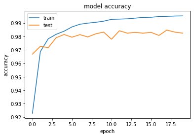
validation_data=(x_test, y_test)でテストデータを指定します。エポックごとに、訓練データとテストデータでの正答率を計算します。それらの戻り値をhistoryで受けています。上記のコードを実行すると、以下のように、エポックごとに学習の計算結果が表示されます。
Using TensorFlow backend.
_________________________________________________________________
Train on 60000 samples, validate on 10000 samples
Epoch 1/20
60000/60000 [==============================] - 15s 255us/step - loss: 0.2500 - acc: 0.9237 - val_loss: 0.1023 - val_acc: 0.9679
Epoch 2/20
60000/60000 [==============================] - 17s 278us/step - loss: 0.1039 - acc: 0.9680 - val_loss: 0.0825 - val_acc: 0.9752
Epoch 3/20
60000/60000 [==============================] - 19s 310us/step - loss: 0.0761 - acc: 0.9775 - val_loss: 0.0712 - val_acc: 0.9797
Epoch 4/20
60000/60000 [==============================] - 18s 293us/step - loss: 0.0618 - acc: 0.9819 - val_loss: 0.0691 - val_acc: 0.9833
Epoch 5/20

---

val_loss: 0.1033 - val_acc: 0.9846
Test loss: 0.10328161851
Test accuracy: 0.9846
このhistoryの中にはそれまでの学習の経過が入っているので、matplotlibで表示してみましょう。
#accuracy
plt.plot(history.history['acc'])
plt.plot(history.history['val_acc'])
plt.title('model accuracy')
plt.ylabel('accuracy')
plt.xlabel('epoch')
plt.legend(['train', 'test'], loc='upper left')
plt.show()

#loss
plt.plot(history.history['loss'])
plt.plot(history.history['val_loss'])
plt.title('model loss')
plt.ylabel('loss')
plt.xlabel('epoch')
plt.legend(['train', 'test'], loc='upper left')
plt.show()
'''Trains a simple deep NN on the MNIST dataset.
Gets to 98.40% test accuracy after 20 epochs
(there is *a lot* of margin for parameter tuning).
2 seconds per epoch on a K520 GPU.
'''

from __future__ import print_function

import keras
from keras.datasets import mnist
from keras.models import Sequential
from keras.layers import Dense, Dropout
from keras.optimizers import RMSprop

batch_size = 128
num_classes = 10
epochs = 20

# the data, split between train and test sets
(x_train, y_train), (x_test, y_test) = mnist.load_data()

x_train = x_train.reshape(60000, 784)
x_test = x_test.reshape(10000, 784)
x_train = x_train.astype('float32')
x_test = x_test.astype('float32')
x_train /= 255
x_test /= 255
print(x_train.shape[0], 'train samples')
print(x_test.shape[0], 'test samples')

# convert class vectors to binary class matrices
y_train = keras.utils.to_categorical(y_train, num_classes)
y_test = keras.utils.to_categorical(y_test, num_classes)

model = Sequential()
model.add(Dense(512, activation='relu', input_shape=(784,)))
model.add(Dropout(0.2))
model.add(Dense(512, activation='relu'))
model.add(Dropout(0.2))
model.add(Dense(num_classes, activation='softmax'))

model.summary()

model.compile(loss='categorical_crossentropy',
              optimizer=RMSprop(),
              metrics=['accuracy'])

history = model.fit(x_train, y_train,
                    batch_size=batch_size,
                    epochs=epochs,
                    verbose=1,
                    validation_data=(x_test, y_test))
score = model.evaluate(x_test, y_test, verbose=0)
print('Test loss:', score[0])
print('Test accuracy:', score[1])
このスクリプトのソースコードはKeras-teamのgithubにある mnist_mlp.pyという名称のexamplesファイルの一つです。
CNNを用いた手書き数字の識別学習モデル |
次に、CNNを使って画像を認識するモデルを構築しましょう。
先ほどは、画像の画素値を、そのまま特徴量として使いました。そのため2次元のデータを1次元に変換したのですが、こう変換してしまうと、上下左右の画素値同士の関係性は考慮されなくなります。 ディープラーニングで画像認識する場合には、一般的にCNN(Convolutional Neural Network、畳み込みニューラルネットワーク)を使います。これにより空間的な特徴を捉えることができます。 Conv2Dメソッドでは、kernel_sizeで指定した範囲の画像を見て、畳み込みを行っています。画像における畳み込み計算は、簡単にいうとフィルター(カーネル)処理です。詳しくは、Deep Learningと人工知能のページを参照してください。
'''Trains a simple convnet on the MNIST dataset.
Gets to 99.25% test accuracy after 12 epochs
(there is still a lot of margin for parameter tuning).
16 seconds per epoch on a GRID K520 GPU.
'''

from __future__ import print_function
import keras
from keras.datasets import mnist
from keras.models import Sequential
from keras.layers import Dense, Dropout, Flatten
from keras.layers import Conv2D, MaxPooling2D
from keras import backend as K

batch_size = 128
num_classes = 10
epochs = 12

# input image dimensions
img_rows, img_cols = 28, 28

# the data, split between train and test sets
(x_train, y_train), (x_test, y_test) = mnist.load_data()

if K.image_data_format() == 'channels_first':
    x_train = x_train.reshape(x_train.shape[0], 1, img_rows, img_cols)
    x_test = x_test.reshape(x_test.shape[0], 1, img_rows, img_cols)
    input_shape = (1, img_rows, img_cols)
else:
    x_train = x_train.reshape(x_train.shape[0], img_rows, img_cols, 1)
    x_test = x_test.reshape(x_test.shape[0], img_rows, img_cols, 1)
    input_shape = (img_rows, img_cols, 1)

x_train = x_train.astype('float32')
x_test = x_test.astype('float32')
x_train /= 255
x_test /= 255
print('x_train shape:', x_train.shape)
print(x_train.shape[0], 'train samples')
print(x_test.shape[0], 'test samples')

# convert class vectors to binary class matrices
y_train = keras.utils.to_categorical(y_train, num_classes)
y_test = keras.utils.to_categorical(y_test, num_classes)

model = Sequential()
model.add(Conv2D(32, kernel_size=(3, 3),
                 activation='relu',
                 input_shape=input_shape))
model.add(Conv2D(64, (3, 3), activation='relu'))
model.add(MaxPooling2D(pool_size=(2, 2)))
model.add(Dropout(0.25))
model.add(Flatten())
model.add(Dense(128, activation='relu'))
model.add(Dropout(0.5))
model.add(Dense(num_classes, activation='softmax'))

model.compile(loss=keras.losses.categorical_crossentropy,
              optimizer=keras.optimizers.Adadelta(),
              metrics=['accuracy'])

model.fit(x_train, y_train,
          batch_size=batch_size,
          epochs=epochs,
          verbose=1,
          validation_data=(x_test, y_test))
score = model.evaluate(x_test, y_test, verbose=0)
print('Test loss:', score[0])
print('Test accuracy:', score[1])
このスクリプトを実行すると、以下のように、計算結果が時間の経過とともに表示がされます。
Using TensorFlow backend.
x_train shape: (60000, 28, 28, 1)
60000 train samples
10000 test samples
Train on 60000 samples, validate on 10000 samples
Epoch 1/12
60000/60000 [==============================] - 147s 2ms/step - loss: 0.2611 - acc: 0.9198 - val_loss: 0.0709 - val_acc: 0.9780
Epoch 2/12
60000/60000 [==============================] - 157s 3ms/step - loss: 0.0884 - acc: 0.9739 - val_loss: 0.0391 - val_acc: 0.9865
Epoch 3/12
60000/60000 [==============================] - 156s 3ms/step - loss: 0.0641 - acc: 0.9805 - val_loss: 0.0338 - val_acc: 0.9889
Epoch 4/12
60000/60000 [==============================] - 143s 2ms/step - loss: 0.0541 - acc: 0.9838 - val_loss: 0.0351 - val_acc: 0.9881
Epoch 5/12
60000/60000 [==============================] - 142s 2ms/step - loss: 0.0474 - acc: 0.9854 - val_loss: 0.0302 - val_acc: 0.9901
Epoch 6/12
60000/60000 [==============================] - 142s 2ms/step - loss: 0.0404 - acc: 0.9882 - val_loss: 0.0267 - val_acc: 0.9909
Epoch 7/12
60000/60000 [==============================] - 144s 2ms/step - loss: 0.0377 - acc: 0.9881 - val_loss: 0.0267 - val_acc: 0.9909
Epoch 8/12
60000/60000 [==============================] - 141s 2ms/step - loss: 0.0321 - acc: 0.9899 - val_loss: 0.0300 - val_acc: 0.9907
Epoch 9/12
60000/60000 [==============================] - 141s 2ms/step - loss: 0.0300 - acc: 0.9907 - val_loss: 0.0283 - val_acc: 0.9912
Epoch 10/12
60000/60000 [==============================] - 141s 2ms/step - loss: 0.0278 - acc: 0.9914 - val_loss: 0.0266 - val_acc: 0.9913
Epoch 11/12
60000/60000 [==============================] - 143s 2ms/step - loss: 0.0255 - acc: 0.9917 - val_loss: 0.0282 - val_acc: 0.9908
Epoch 12/12
60000/60000 [==============================] - 220s 4ms/step - loss: 0.0253 - acc: 0.9918 - val_loss: 0.0350 - val_acc: 0.9898
Test loss: 0.035007441200863104
Test accuracy: 0.9898
通常のPCでは30分程度かかります。テストデータでの正答率が98.98%という結果になりました。 先ほどのCNNを使わない試行では最高の正答率が98.47%だったので、精度が向上しました。
from keras.datasets import cifar10
(x_train, y_train), (x_test, y_test) = cifar10.load_data()
と入力します。 戻り値は2つのタプルからなります。
このコードを実行すると1回のepochに数時間かかります。時間に余裕があるときに実行して見てください。
学習済みモデルを用いた画像からの物体の識別 |
通常のCPUを搭載したPCでは、正答率が90%を超えるまでニューラルネットワークの学習を行うためには、数時間から数日も必要とされます。Kerasには、学習済みモデルが用意されています。ImageNetで学習した重みをもつ画像分類のモデルとして、以下のものが用意されています。
Xception
VGG16
VGG19
ResNet50
InceptionV3
InceptionResNetV2
MobileNet
DenseNet
NASNet
from keras.applications.vgg16 import VGG16
from keras.preprocessing import image
from keras.applications.vgg16 import preprocess_input, decode_predictions
import numpy as np
model = VGG16(include_top=True, weights='imagenet', input_tensor=None, input_shape=None)
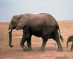
img_path = 'images/elephant.jpg'
img = image.load_img(img_path, target_size=(224, 224))
x = image.img_to_array(img)
x = np.expand_dims(x, axis=0)
x = preprocess_input(x)
model.summary()
preds = model.predict(x)
# decode the results into a list of tuples (class, description, probability)
# (one such list for each sample in the batch)
print('Predicted:', decode_predictions(preds, top=3)[0])
Using TensorFlow backend.
Layer (type)                 Output Shape              Param #
=================================================================
input_1 (InputLayer)         (None, 224, 224, 3)       0
_________________________________________________________________
block1_conv1 (Conv2D)        (None, 224, 224, 64)      1792
_________________________________________________________________
block1_conv2 (Conv2D)        (None, 224, 224, 64)      36928
_________________________________________________________________
block1_pool (MaxPooling2D)   (None, 112, 112, 64)      0
_________________________________________________________________
block2_conv1 (Conv2D)        (None, 112, 112, 128)     73856
_________________________________________________________________
block2_conv2 (Conv2D)        (None, 112, 112, 128)     147584
_________________________________________________________________
block2_pool (MaxPooling2D)   (None, 56, 56, 128)       0
_________________________________________________________________
block3_conv1 (Conv2D)        (None, 56, 56, 256)       295168
_________________________________________________________________
block3_conv2 (Conv2D)        (None, 56, 56, 256)       590080
_________________________________________________________________
block3_conv3 (Conv2D)        (None, 56, 56, 256)       590080
_________________________________________________________________
block3_pool (MaxPooling2D)   (None, 28, 28, 256)       0
_________________________________________________________________
block4_conv1 (Conv2D)        (None, 28, 28, 512)       1180160
_________________________________________________________________
block4_conv2 (Conv2D)        (None, 28, 28, 512)       2359808
_________________________________________________________________
block4_conv3 (Conv2D)        (None, 28, 28, 512)       2359808
_________________________________________________________________
block4_pool (MaxPooling2D)   (None, 14, 14, 512)       0
_________________________________________________________________
block5_conv1 (Conv2D)        (None, 14, 14, 512)       2359808
_________________________________________________________________
block5_conv2 (Conv2D)        (None, 14, 14, 512)       2359808
_________________________________________________________________
block5_conv3 (Conv2D)        (None, 14, 14, 512)       2359808
_________________________________________________________________
block5_pool (MaxPooling2D)   (None, 7, 7, 512)         0
_________________________________________________________________
flatten (Flatten)            (None, 25088)             0
_________________________________________________________________
fc1 (Dense)                  (None, 4096)              102764544
_________________________________________________________________
fc2 (Dense)                  (None, 4096)              16781312
_________________________________________________________________
predictions (Dense)          (None, 1000)              4097000
=================================================================
Total params: 138,357,544
Trainable params: 138,357,544
Non-trainable params: 0
_________________________________________________________________
Predicted: [('n02504458', 'African_elephant', 0.7639994), ('n01871265', 'tusker', 0.173594), ('n02504013', 'Indian_elephant', 0.062363632)]
from keras.applications.resnet50 import ResNet50
from keras.preprocessing import image
from keras.applications.resnet50 import preprocess_input, decode_predictions
import numpy as np

model = ResNet50(weights='imagenet')

img_path = 'images/elephant.jpg'
img = image.load_img(img_path, target_size=(224, 224))
x = image.img_to_array(img)
x = np.expand_dims(x, axis=0)
x = preprocess_input(x)

preds = model.predict(x)

# decode the results into a list of tuples (class, description, probability)
# (one such list for each sample in the batch)
print('Predicted:', decode_predictions(preds, top=3)[0])
Using TensorFlow backend.
Predicted: [('n02504458', 'African_elephant', 0.8089608), ('n01871265', 'tusker', 0.12518124), ('n02504013', 'Indian_elephant', 0.064179957)]
from keras.applications.inception_v3 import InceptionV3
from keras.preprocessing import image
from keras.applications.inception_v3 import preprocess_input, decode_predictions
import numpy as np

model = InceptionV3(weights='imagenet')

img_path = 'images/elephant.jpg'
img = image.load_img(img_path, target_size=(299, 299))
x = image.img_to_array(img)
x = np.expand_dims(x, axis=0)
x = preprocess_input(x)

preds = model.predict(x)

# decode the results into a list of tuples (class, description, probability)
# (one such list for each sample in the batch)
print('Predicted:', decode_predictions(preds, top=3)[0])
Predicted: [('n02504458', 'African_elephant', 0.61769462), ('n01871265', 'tusker', 0.31645635), ('n02504013', 'Indian_elephant', 0.032580622)]